In this post, we create a simple convolutional neural network(SimpeConvNet) using only NumPy and…

Simple CovNet with NumPy

In this post, we create a simple convolutional neural network(SimpeConvNet) using only NumPy and it will classify MNIST images. The codes are from a book called ‘Deep Learning from Scratch’. Let’s check an architecture of SimpeConvNet and notations first.

Architecture

N: the number of images (or mini batch size)

H: the height of images

W: the width of images

FN: the number of filters

FH: the height of filters

FW: the width of filters

C: the depth of channel

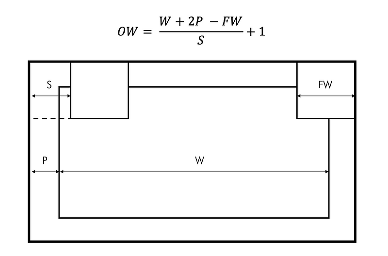
OH: the height of outputs

OW: the width of outputs

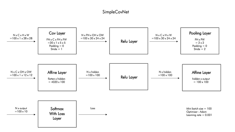
The architecture of simple convolution network is from the convolution layer to the softmax with loss layer. You can find source codes here and explanation of them from my posts: Convolution, Pool, Affine, Relu, Softmax with Loss.

The forward pass of convolutional layer produces a four-dimensional tensor with[N, FN, OH, OW] shape, where FNcorresponds to the number of filters applied in a given layer. The output size of convolution is (28 + 2x0–5) / 1 + 1 that is 24.

The pooling layer transforms the tensor form original shape [N, C, H, W]to [N, C, OH, OW]. Here the ratio between H and OH is defined by stride and pool_size hyperparameters. The output size of pooling layer is 20 x (24/2) x (24/2) that is 4320.

Simple ConvNet

You need to visit Github for imports, auxiliary functions and MNIST dataset. There are 7 layers that are Conv1, Relu1, Pool1, Affine 1, Relu2, Affine 2 and Softmax with Loss.

Before we compute the loss, we need to first perform a forward pass. It takes the values of layers(conv — relu — pool — affine — relu — affine) and forward them. As we defined the last layer is the softmax and loss layer, we will be using the cross-entropy loss.

The accuracy is calculated by dividing the number of correct answers by the number of data.

It starts by computing the forward over all the layers, then computes the error between the output of the network and the target value. We can make grads dictionary by using backward function of each layer in reverse order, starting by the last one up to the first.

This can be used when you want use trained parameters.

Train Simple ConvNet

After reading data, we reduce the number data since it might take too much time training and then set parameters. For training, we use a trainer that you can find its code of here and change the optimizer. The options are ‘sgd’, ‘momentum’, ‘nesterov’, ‘adagrad’, ‘rmsprpo’ and ‘adam’. You can read the explanation of some of them here.

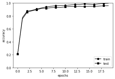
The below is the graph of history of accuracy while training.

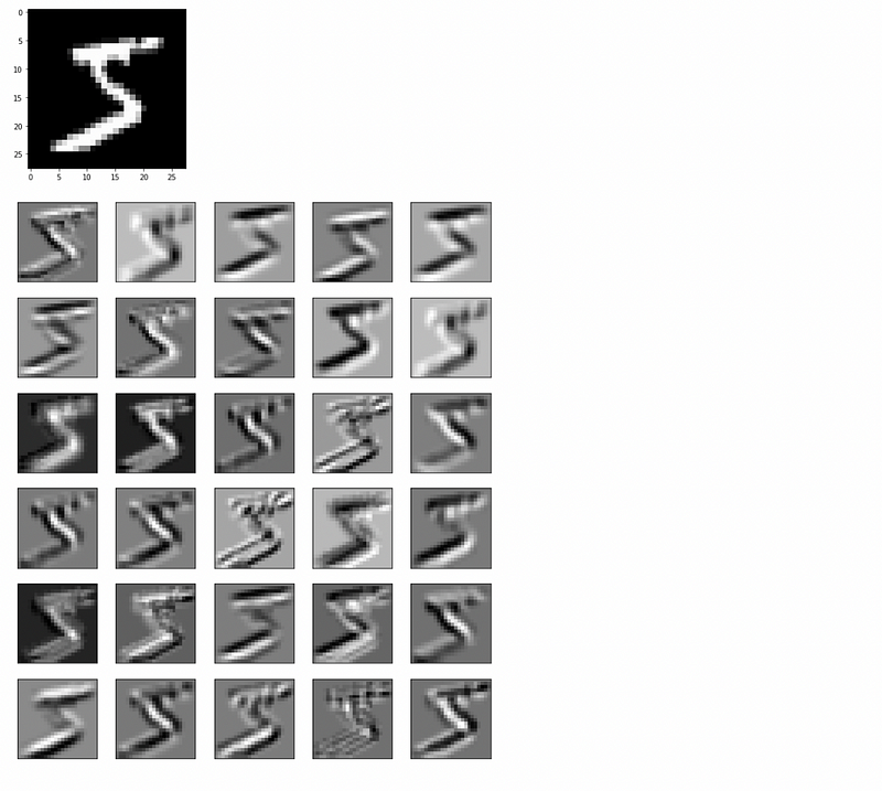
Apply Filter to MNIST

We can use the ‘params.pk’ file by using load_params function so that we can visualize trained filters. Since we set the number of filters as 30, we can apply 30 filters into each image. Each filter has local features.

I hope that my post has broadened your horizons and increased your understanding of operations of convolution network. Thank you for reading :)