Google ISLR Transformer with W&B (Part 2)
In this article, I’ll be showing you how to create and train a model for the Kaggle ASL (American Sign Language) recognition competition…

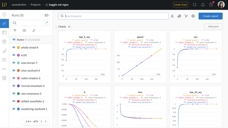
In this article, I’ll be showing you how to create and train a model for the Kaggle ASL (American Sign Language) recognition competition, building on my previous post. I’ve used and modified Mark Wijkhuizen’s code and monitored the training process using W&B, and you can check out the full code and my W&B dashboard in this article. Let’s dive in!
Global Config & Utils
cfg = SimpleNamespace()
# If True, processing data from scratch
# If False, loads preprocessed data
cfg.PREPROCESS_DATA = False
cfg.TRAIN_MODEL = True
# True: use 10% of participants as validation set
# False: use all data for training
cfg.USE_VAL = False

cfg.N_ROWS = 543
cfg.N_DIMS = 3
cfg.DIM_NAMES = ['x', 'y', 'z']
cfg.SEED = 42
cfg.NUM_CLASSES = 250

cfg.IS_INTERACTIVE = True
cfg.VERBOSE = 2
cfg.INPUT_SIZE = 64

cfg.BATCH_ALL_SIGNS_N = 4
cfg.BATCH_SIZE = 256
cfg.N_EPOCHS = 100
cfg.LR_MAX = 1e-3
cfg.N_WARMUP_EPOCHS = 0

# Dropout Ratio
cfg.WD_RATIO = 0.05

#cfg.MASK_VAL = 4237
Here’s an explanation of the parameters in cfg:
PREPROCESS_DATA: a boolean value that indicates whether to process data from scratch or to load preprocessed dataTRAIN_MODEL: a boolean value that indicates whether to train the model or notUSE_VAL: a boolean value that indicates whether to use 10% of participants as a validation set or to use all data for trainingN_ROWS: the number of rows in the input datasetN_DIMS: the number of dimensions in the input datasetDIM_NAMES: a list of strings that represents the names of the dimensions in the input datasetSEED: the random seed for reproducibilityNUM_CLASSES: the number of classes in the outputIS_INTERACTIVE: a boolean value that indicates whether to run in interactive modeVERBOSE: the verbosity level (0 = silent, 1 = progress bar, 2 = one line per epoch)INPUT_SIZE: the input size for the model. If the input size is bigger, it can provide more information to the model, and the model can learn more complex and accurate representations of the input data. However, I experienced a SCORING ERROR when I increased it to 128. It’s probably because the increased INPUT_SIZE exceeded the model size required for this competition.BATCH_ALL_SIGNS_N: the number of signs to use in each batch during trainingBATCH_SIZE: the batch size for trainingN_EPOCHS: the number of epochs to trainLR_MAX: the maximum learning rate for the one-cycle learning rate policyN_WARMUP_EPOCHS: the number of warm-up epochs for the one-cycle learning rate policyWD_RATIO: the weight decay ratioMASK_VAL: a value used for masking, but commented out in this code block
Model Config
# Epsilon value for layer normalisation
LAYER_NORM_EPS = 1e-6

# Dense layer units for landmarks
LIPS_UNITS = 384
HANDS_UNITS = 384
POSE_UNITS = 384

# Final embedding and transformer embedding size
UNITS = 512

# Transformer
NUM_BLOCKS = 2
MLP_RATIO = 2

# Dropout
EMBEDDING_DROPOUT = 0.00
MLP_DROPOUT_RATIO = 0.30
CLASSIFIER_DROPOUT_RATIO = 0.10

# Initiailizers
INIT_HE_UNIFORM = tf.keras.initializers.he_uniform
INIT_GLOROT_UNIFORM = tf.keras.initializers.glorot_uniform
INIT_ZEROS = tf.keras.initializers.constant(0.0)

# Activations
GELU = tf.keras.activations.gelu

print(f'UNITS: {UNITS}')

'''
UNITS: 512
'''
Firstly, we define various hyperparameters and print the value of UNITS. Let’s dive into the hyperparameters used:
- LAYER_NORM_EPS: This is a small value added to the denominator in the Layer Normalization operation to avoid division by zero. In this case, the value used is 1e-6.
- LIPS_UNITS, HANDS_UNITS, and POSE_UNITS: These are the number of units in the Dense layers used to extract features from the landmarks of the lips, hands, and pose, respectively. The values used are 384 for each.
- UNITS: This is the size of the final embedding and the transformer embedding. In this case, the value used is 512, which is the size of the final embedding and transformer embedding. This means that each input token will be represented by a vector of size 512. The performance of the model may be affected by the choice of this hyperparameter, as increasing the size of the embeddings may improve the model’s ability to capture complex relationships between input tokens, but may also lead to overfitting or increased computation time.
- NUM_BLOCKS: This is the number of Transformer blocks used in the model. In this case, the value used is 2. Increasing the number of blocks can allow for more complex and nuanced representations of the input data, potentially leading to improved accuracy on tasks such as natural language processing or image recognition.
- MLP_RATIO: This is the ratio of the number of hidden units in the Feedforward network of the Transformer block to the number of input units. In this case, the value used is 2.
- EMBEDDING_DROPOUT: This is the dropout rate applied to the input embeddings. In this case, no dropout is applied.
- MLP_DROPOUT_RATIO: This is the dropout rate applied to the output of the Feedforward network in the Transformer block. In this case, a dropout rate of 30% is used.
- CLASSIFIER_DROPOUT_RATIO: This is the dropout rate applied to the output of the final classifier. In this case, a dropout rate of 10% is used.
- INIT_HE_UNIFORM: This is the initializer used for the kernel weights in the Dense layers. In this case, the He uniform initializer is used.
- INIT_GLOROT_UNIFORM: This is the initializer used for the kernel weights in the Transformer blocks. In this case, the Glorot uniform initializer is used.
- INIT_ZEROS: This is the initializer used for the bias terms in the Dense layers. In this case, the constant initializer with a value of 0.0 is used.
- GELU: This is the activation function used in the Feedforward network of the Transformer block. In this case, the Gaussian Error Linear Units (GELU) activation function is used.
Transformer
The encoder part of the model consists of N identical layers, each of which can be further divided into the following steps:
- Embedding of the one-hot encoded input sample (word embedding)
- Addition of position encoding
- Multi-head self-attention mechanism
- Addition of the input and output of self-attention (residual network structure)
- Layer normalization of all time steps
- Feedforward neural network structure
- Addition of the input and output of the feedforward network (residual network structure)
- Layer normalization of all time steps
- Repeat steps 3–8 for N layers
The decoder part of the model is also N identical layers, each of which can be further divided into the following steps:
- Embedding of the one-hot encoded input sample (word embedding)
- Addition of position encoding
- Multi-head self-attention mechanism
- Addition of the input and output of self-attention (residual network structure)
- Layer normalization of all time steps
- Multi-head cross-attention mechanism with the encoder output as queries and keys and the previous decoder layer output as values
- Addition of the input and output of cross-attention (residual network structure)
- Layer normalization of all time steps
- Feedforward neural network structure
- Addition of the input and output of the feedforward network (residual network structure)
- Layer normalization of all time steps
- Repeat steps 3–11 for N layers
The output of the model is generated by passing the final output through a linear layer followed by a softmax activation function for prediction.
We need to use the scaled dot-product attention between the queries q, keys k, and values v for MultiHeadAttention. The function computes the weighted sum of the values using the attention scores by using tf.matmul with softmax and v. The output tensor has the same shape as the inputs q, k, and v.
# based on: https://stackoverflow.com/questions/67342988/verifying-the-implementation-of-multihead-attention-in-transformer
# replaced softmax with softmax layer to support masked softmax

def scaled_dot_product(q,k,v, softmax, attention_mask):
    #calculates Q . K(transpose)
    qkt = tf.matmul(q,k,transpose_b=True)
    #caculates scaling factor
    dk = tf.math.sqrt(tf.cast(q.shape[-1],dtype=tf.float32))
    scaled_qkt = qkt/dk
    softmax = softmax(scaled_qkt, mask=attention_mask)

    z = tf.matmul(softmax,v)
    #shape: (m,Tx,depth), same shape as q,k,v
    return z
As an important component, MultiHeadAttention is implemented. It takes in d_model and num_of_heads arguments.
class MultiHeadAttention(tf.keras.layers.Layer):
    def __init__(self,d_model,num_of_heads):
        super(MultiHeadAttention,self).__init__()
        self.d_model = d_model
        self.num_of_heads = num_of_heads
        self.depth = d_model//num_of_heads
        self.wq = [tf.keras.layers.Dense(self.depth) for i in range(num_of_heads)]
        self.wk = [tf.keras.layers.Dense(self.depth) for i in range(num_of_heads)]
        self.wv = [tf.keras.layers.Dense(self.depth) for i in range(num_of_heads)]
        self.wo = tf.keras.layers.Dense(d_model)
        self.softmax = tf.keras.layers.Softmax()

    def call(self,x, attention_mask):

        multi_attn = []
        for i in range(self.num_of_heads):
            Q = self.wq[i](x)
            K = self.wk[i](x)
            V = self.wv[i](x)
            multi_attn.append(scaled_dot_product(Q,K,V, self.softmax, attention_mask))

        multi_head = tf.concat(multi_attn,axis=-1)
        multi_head_attention = self.wo(multi_head)
        return multi_head_attention
# Full Transformer
class Transformer(tf.keras.Model):
def __init__(self, num_blocks):
super(Transformer, self).__init__(name='transformer')
self.num_blocks = num_blocks
def build(self, input_shape):
self.ln_1s = []
self.mhas = []
self.ln_2s = []
self.mlps = []
# Make Transformer Blocks
for i in range(self.num_blocks):
# Multi Head Attention
self.mhas.append(MultiHeadAttention(UNITS, 8))
# Multi Layer Perception
self.mlps.append(tf.keras.Sequential([
tf.keras.layers.Dense(UNITS * MLP_RATIO, activation=GELU, kernel_initializer=INIT_GLOROT_UNIFORM),
tf.keras.layers.Dropout(MLP_DROPOUT_RATIO),
tf.keras.layers.Dense(UNITS, kernel_initializer=INIT_HE_UNIFORM),
]))
def call(self, x, attention_mask):
# Iterate input over transformer blocks
for mha, mlp in zip(self.mhas, self.mlps):
x = x + mha(x, attention_mask)
x = x + mlp(x)
return xEmbedding
Embedding is a learned representation of a categorical variable. In the Embedding class, the LandmarkEmbedding is used to embed the landmark data. The output of each LandmarkEmbedding is concatenated along the last dimension.
Landmark Embedding
The goal of LandmarkEmbedding is to represent landmark data in a continuous vector space, so that it can be easily used as input to downstream machine models.
The dense layer learns a representation of the landmark data by mapping it to a continuous vector space. This allows the downstream models to extract relevant features from the landmark data.
It also handles missing landmarks by providing a separate embedding for frames where certain landmarks are missing.
class LandmarkEmbedding(tf.keras.Model):
    def __init__(self, units, name):
        super(LandmarkEmbedding, self).__init__(name=f'{name}_embedding')
        self.units = units

    def build(self, input_shape):
        # Embedding for missing landmark in frame, initizlied with zeros
        self.empty_embedding = self.add_weight(
            name=f'{self.name}_empty_embedding',
            shape=[self.units],
            initializer=INIT_ZEROS,
        )
        # Embedding
        self.dense = tf.keras.Sequential([
            tf.keras.layers.Dense(self.units, name=f'{self.name}_dense_1', use_bias=False, kernel_initializer=INIT_GLOROT_UNIFORM),
            tf.keras.layers.Activation(GELU),
            tf.keras.layers.Dense(self.units, name=f'{self.name}_dense_2', use_bias=False, kernel_initializer=INIT_HE_UNIFORM),
        ], name=f'{self.name}_dense')

    def call(self, x):
        return tf.where(
                # Checks whether landmark is missing in frame
                tf.reduce_sum(x, axis=2, keepdims=True) == 0,
                # If so, the empty embedding is used
                self.empty_embedding,
                # Otherwise the landmark data is embedded
                self.dense(x),
            )
Embedding
The purpose of Embedding is to embed various types of input data, such as lip landmark coordinates.
The positional embedding layer is initialized with zeros and is used to add positional information to the landmark embeddings. The weights for each type of landmark embedding are initialized with zeros and are learned during training. The fully connected layer is used to combine the embeddings of all landmarks.
class Embedding(tf.keras.Model):
    def __init__(self):
        super(Embedding, self).__init__()

    def get_diffs(self, l):
        S = l.shape[2]
        other = tf.expand_dims(l, 3)
        other = tf.repeat(other, S, axis=3)
        other = tf.transpose(other, [0,1,3,2])
        diffs = tf.expand_dims(l, 3) - other
        diffs = tf.reshape(diffs, [-1, cfg.INPUT_SIZE, S*S])
        return diffs

    def build(self, input_shape):
        # Positional Embedding, initialized with zeros
        self.positional_embedding = tf.keras.layers.Embedding(cfg.INPUT_SIZE+1, UNITS, embeddings_initializer=INIT_ZEROS)
        # Embedding layer for Landmarks
        self.lips_embedding = LandmarkEmbedding(LIPS_UNITS, 'lips')
        self.left_hand_embedding = LandmarkEmbedding(HANDS_UNITS, 'left_hand')
        self.pose_embedding = LandmarkEmbedding(POSE_UNITS, 'pose')
        # Landmark Weights
        self.landmark_weights = tf.Variable(tf.zeros([3], dtype=tf.float32), name='landmark_weights')
        # Fully Connected Layers for combined landmarks
        self.fc = tf.keras.Sequential([
            tf.keras.layers.Dense(UNITS, name='fully_connected_1', use_bias=False, kernel_initializer=INIT_GLOROT_UNIFORM),
            tf.keras.layers.Activation(GELU),
            tf.keras.layers.Dense(UNITS, name='fully_connected_2', use_bias=False, kernel_initializer=INIT_HE_UNIFORM),
        ], name='fc')


    def call(self, lips0, left_hand0, pose0, non_empty_frame_idxs, training=False):
        # Lips
        lips_embedding = self.lips_embedding(lips0)
        # Left Hand
        left_hand_embedding = self.left_hand_embedding(left_hand0)
        # Pose
        pose_embedding = self.pose_embedding(pose0)
        # Merge Embeddings of all landmarks with mean pooling
        x = tf.stack((
            lips_embedding, left_hand_embedding, pose_embedding,
        ), axis=3)
        x = x * tf.nn.softmax(self.landmark_weights)
        x = tf.reduce_sum(x, axis=3)
        # Fully Connected Layers
        x = self.fc(x)
        # Add Positional Embedding
        max_frame_idxs = tf.clip_by_value(
                tf.reduce_max(non_empty_frame_idxs, axis=1, keepdims=True),
                1,
                np.PINF,
            )
        normalised_non_empty_frame_idxs = tf.where(
            tf.math.equal(non_empty_frame_idxs, -1.0),
            cfg.INPUT_SIZE,
            tf.cast(
                non_empty_frame_idxs / max_frame_idxs * cfg.INPUT_SIZE,
                tf.int32,
            ),
        )
        x = x + self.positional_embedding(normalised_non_empty_frame_idxs)

        return x
Sparse Categorical Crossentropy With Label Smoothing
Sparse categorical cross-entropy is a loss function used for multi-class classification problems where the labels are integers instead of one-hot encoded vectors.
Label smoothing is a technique used to improve the generalization of a model by preventing it from becoming overconfident in its predictions. It involves smoothing the one-hot encoded target labels by replacing some of the 1’s with a small positive value and the rest with a small negative value.
# source:: https://stackoverflow.com/questions/60689185/label-smoothing-for-sparse-categorical-crossentropy
def scce_with_ls(y_true, y_pred):
    # One Hot Encode Sparsely Encoded Target Sign
    y_true = tf.cast(y_true, tf.int32)
    y_true = tf.one_hot(y_true, cfg.NUM_CLASSES, axis=1)
    y_true = tf.squeeze(y_true, axis=2)
    # Categorical Crossentropy with native label smoothing support
    return tf.keras.losses.categorical_crossentropy(y_true, y_pred, label_smoothing=0.25)
Model
The model takes two inputs: “frames” and “non_empty_frame_idxs”. The “frames” input is a 4D tensor with dimensions [INPUT_SIZE, N_COLS, N_DIMS]. The “non_empty_frame_idxs” input is a 1D tensor with length “INPUT_SIZE”.
- Padding mask: The function first creates a padding mask based on the “non_empty_frame_idxs” input, which is used to mask out any padding frames.
- Normalizing frames: The function then slices the “frames” input into different body parts (lips, left hand, right hand, and pose), normalizes the data using mean and standard deviation values, and reshapes the tensors.
- Embedding: The function then passes the body parts through an “Embedding” layer. This layer learns an embedding representation of the body part data, which is then passed to a Transformer layer with “NUM_BLOCKS” blocks.
- Transformer, Pooling, and Classification: After the Transformer layer, the output is pooled to produce a single vector that is fed into a final dense layer with “NUM_CLASSES” output neurons.
- Model, Loss, and Optimizer: The model is compiled using a categorical cross-entropy loss function and an Adam optimizer with weight decay
- Metrics: There are three metrics: sparse categorical accuracy, sparse top-5 categorical accuracy, and sparse top-10 categorical accuracy.
def get_model():
    # Inputs
    frames = tf.keras.layers.Input([cfg.INPUT_SIZE, N_COLS, cfg.N_DIMS], dtype=tf.float32, name='frames')
    non_empty_frame_idxs = tf.keras.layers.Input([cfg.INPUT_SIZE], dtype=tf.float32, name='non_empty_frame_idxs')
    # Padding Mask
    mask0 = tf.cast(tf.math.not_equal(non_empty_frame_idxs, -1), tf.float32)
    mask0 = tf.expand_dims(mask0, axis=2)
    # Random Frame Masking
    mask = tf.where(
        (tf.random.uniform(tf.shape(mask0)) > 0.25) & tf.math.not_equal(mask0, 0.0),
        1.0,
        0.0,
    )
    # Correct Samples Which are all masked now...
    mask = tf.where(
        tf.math.equal(tf.reduce_sum(mask, axis=[1,2], keepdims=True), 0.0),
        mask0,
        mask,
    )


    """
        left_hand: 468:489
        pose: 489:522
        right_hand: 522:543
    """
    x = frames
    x = tf.slice(x, [0,0,0,0], [-1,cfg.INPUT_SIZE, N_COLS, 2])
    # LIPS
    lips = tf.slice(x, [0,0,LIPS_START,0], [-1,cfg.INPUT_SIZE, 40, 2])
    lips = tf.where(
            tf.math.equal(lips, 0.0),
            0.0,
            (lips - LIPS_MEAN) / LIPS_STD,
        )
    # LEFT HAND
    left_hand = tf.slice(x, [0,0,40,0], [-1,cfg.INPUT_SIZE, 21, 2])
    left_hand = tf.where(
            tf.math.equal(left_hand, 0.0),
            0.0,
            (left_hand - LEFT_HANDS_MEAN) / LEFT_HANDS_STD,
        )
    # POSE
    pose = tf.slice(x, [0,0,61,0], [-1, cfg.INPUT_SIZE, 5, 2])
    pose = tf.where(
            tf.math.equal(pose, 0.0),
            0.0,
            (pose - POSE_MEAN) / POSE_STD,
        )

    # Flatten
    lips = tf.reshape(lips, [-1, cfg.INPUT_SIZE, 40*2])
    left_hand = tf.reshape(left_hand, [-1, cfg.INPUT_SIZE, 21*2])
    pose = tf.reshape(pose, [-1, cfg.INPUT_SIZE, 5*2])

    # Embedding
    x = Embedding()(lips, left_hand, pose, non_empty_frame_idxs)

    # Encoder Transformer Blocks
    x = Transformer(NUM_BLOCKS)(x, mask)

    # Pooling
    x = tf.reduce_sum(x * mask, axis=1) / tf.reduce_sum(mask, axis=1)
    # Classifier Dropout
    x = tf.keras.layers.Dropout(CLASSIFIER_DROPOUT_RATIO)(x)
    # Classification Layer
    x = tf.keras.layers.Dense(cfg.NUM_CLASSES, activation=tf.keras.activations.softmax, kernel_initializer=INIT_GLOROT_UNIFORM)(x)

    outputs = x

    # Create Tensorflow Model
    model = tf.keras.models.Model(inputs=[frames, non_empty_frame_idxs], outputs=outputs)

    # Sparse Categorical Cross Entropy With Label Smoothing
    loss = scce_with_ls

    # Adam Optimizer with weight decay
    optimizer = tfa.optimizers.AdamW(learning_rate=1e-3, weight_decay=1e-5, clipnorm=1.0)

    # TopK Metrics
    metrics = [
        tf.keras.metrics.SparseCategoricalAccuracy(name='acc'),
        tf.keras.metrics.SparseTopKCategoricalAccuracy(k=5, name='top_5_acc'),
        tf.keras.metrics.SparseTopKCategoricalAccuracy(k=10, name='top_10_acc'),
    ]

    model.compile(loss=loss, optimizer=optimizer, metrics=metrics)

    return model
And you can print a summary of the model.
tf.keras.backend.clear_session()
model = get_model()

# Plot model summary
model.summary(expand_nested=True)
Model: "model"
__________________________________________________________________________________________________
Layer (type) Output Shape Param # Connected to
==================================================================================================
non_empty_frame_idxs (InputLay [(None, 64)] 0 []
er)
tf.math.not_equal (TFOpLambda) (None, 64) 0 ['non_empty_frame_idxs[0][0]']
tf.cast (TFOpLambda) (None, 64) 0 ['tf.math.not_equal[0][0]']
tf.expand_dims (TFOpLambda) (None, 64, 1) 0 ['tf.cast[0][0]']
frames (InputLayer) [(None, 64, 66, 3)] 0 []
tf.compat.v1.shape (TFOpLambda (3,) 0 ['tf.expand_dims[0][0]']
)
tf.slice (TFOpLambda) (None, 64, 66, 2) 0 ['frames[0][0]']
tf.random.uniform (TFOpLambda) (None, 64, 1) 0 ['tf.compat.v1.shape[0][0]']
tf.slice_1 (TFOpLambda) (None, 64, 40, 2) 0 ['tf.slice[0][0]']
tf.slice_2 (TFOpLambda) (None, 64, 21, 2) 0 ['tf.slice[0][0]']
tf.slice_3 (TFOpLambda) (None, 64, 5, 2) 0 ['tf.slice[0][0]']
tf.math.greater (TFOpLambda) (None, 64, 1) 0 ['tf.random.uniform[0][0]']
tf.math.not_equal_1 (TFOpLambd (None, 64, 1) 0 ['tf.expand_dims[0][0]']
a)
tf.math.subtract (TFOpLambda) (None, 64, 40, 2) 0 ['tf.slice_1[0][0]']
tf.math.subtract_1 (TFOpLambda (None, 64, 21, 2) 0 ['tf.slice_2[0][0]']
)
tf.math.subtract_2 (TFOpLambda (None, 64, 5, 2) 0 ['tf.slice_3[0][0]']
)
tf.math.logical_and (TFOpLambd (None, 64, 1) 0 ['tf.math.greater[0][0]',
a) 'tf.math.not_equal_1[0][0]']
tf.math.equal_1 (TFOpLambda) (None, 64, 40, 2) 0 ['tf.slice_1[0][0]']
tf.math.truediv (TFOpLambda) (None, 64, 40, 2) 0 ['tf.math.subtract[0][0]']
tf.math.equal_2 (TFOpLambda) (None, 64, 21, 2) 0 ['tf.slice_2[0][0]']
tf.math.truediv_1 (TFOpLambda) (None, 64, 21, 2) 0 ['tf.math.subtract_1[0][0]']
tf.math.equal_3 (TFOpLambda) (None, 64, 5, 2) 0 ['tf.slice_3[0][0]']
tf.math.truediv_2 (TFOpLambda) (None, 64, 5, 2) 0 ['tf.math.subtract_2[0][0]']
tf.where (TFOpLambda) (None, 64, 1) 0 ['tf.math.logical_and[0][0]']
tf.where_2 (TFOpLambda) (None, 64, 40, 2) 0 ['tf.math.equal_1[0][0]',
'tf.math.truediv[0][0]']
tf.where_3 (TFOpLambda) (None, 64, 21, 2) 0 ['tf.math.equal_2[0][0]',
'tf.math.truediv_1[0][0]']
tf.where_4 (TFOpLambda) (None, 64, 5, 2) 0 ['tf.math.equal_3[0][0]',
'tf.math.truediv_2[0][0]']
tf.math.reduce_sum (TFOpLambda (None, 1, 1) 0 ['tf.where[0][0]']
)
tf.reshape (TFOpLambda) (None, 64, 80) 0 ['tf.where_2[0][0]']
tf.reshape_1 (TFOpLambda) (None, 64, 42) 0 ['tf.where_3[0][0]']
tf.reshape_2 (TFOpLambda) (None, 64, 10) 0 ['tf.where_4[0][0]']
tf.math.equal (TFOpLambda) (None, 1, 1) 0 ['tf.math.reduce_sum[0][0]']
embedding (Embedding) (None, 64, 512) 986243 ['tf.reshape[0][0]',
'tf.reshape_1[0][0]',
'tf.reshape_2[0][0]',
'non_empty_frame_idxs[0][0]']
|¯¯¯¯¯¯¯¯¯¯¯¯¯¯¯¯¯¯¯¯¯¯¯¯¯¯¯¯¯¯¯¯¯¯¯¯¯¯¯¯¯¯¯¯¯¯¯¯¯¯¯¯¯¯¯¯¯¯¯¯¯¯¯¯¯¯¯¯¯¯¯¯¯¯¯¯¯¯¯¯¯¯¯¯¯¯¯¯¯¯¯¯¯¯¯¯|
| embedding (Embedding) multiple 33280 [] |
| |
| lips_embedding (LandmarkEmbedd multiple 178560 [] |
| ing) |
||¯¯¯¯¯¯¯¯¯¯¯¯¯¯¯¯¯¯¯¯¯¯¯¯¯¯¯¯¯¯¯¯¯¯¯¯¯¯¯¯¯¯¯¯¯¯¯¯¯¯¯¯¯¯¯¯¯¯¯¯¯¯¯¯¯¯¯¯¯¯¯¯¯¯¯¯¯¯¯¯¯¯¯¯¯¯¯¯¯¯¯¯¯¯||
|| lips_embedding_dense (Sequenti (None, 64, 384) 178176 [] ||
|| al) ||
|||¯¯¯¯¯¯¯¯¯¯¯¯¯¯¯¯¯¯¯¯¯¯¯¯¯¯¯¯¯¯¯¯¯¯¯¯¯¯¯¯¯¯¯¯¯¯¯¯¯¯¯¯¯¯¯¯¯¯¯¯¯¯¯¯¯¯¯¯¯¯¯¯¯¯¯¯¯¯¯¯¯¯¯¯¯¯¯¯¯¯¯¯|||
||| lips_embedding_dense_1 (Dense) (None, 64, 384) 30720 [] |||
||| |||
||| activation_1 (Activation) (None, 64, 384) 0 [] |||
||| |||
||| lips_embedding_dense_2 (Dense) (None, 64, 384) 147456 [] |||
||¯¯¯¯¯¯¯¯¯¯¯¯¯¯¯¯¯¯¯¯¯¯¯¯¯¯¯¯¯¯¯¯¯¯¯¯¯¯¯¯¯¯¯¯¯¯¯¯¯¯¯¯¯¯¯¯¯¯¯¯¯¯¯¯¯¯¯¯¯¯¯¯¯¯¯¯¯¯¯¯¯¯¯¯¯¯¯¯¯¯¯¯¯¯||
|¯¯¯¯¯¯¯¯¯¯¯¯¯¯¯¯¯¯¯¯¯¯¯¯¯¯¯¯¯¯¯¯¯¯¯¯¯¯¯¯¯¯¯¯¯¯¯¯¯¯¯¯¯¯¯¯¯¯¯¯¯¯¯¯¯¯¯¯¯¯¯¯¯¯¯¯¯¯¯¯¯¯¯¯¯¯¯¯¯¯¯¯¯¯¯¯|
| left_hand_embedding (LandmarkE multiple 163968 [] |
| mbedding) |
||¯¯¯¯¯¯¯¯¯¯¯¯¯¯¯¯¯¯¯¯¯¯¯¯¯¯¯¯¯¯¯¯¯¯¯¯¯¯¯¯¯¯¯¯¯¯¯¯¯¯¯¯¯¯¯¯¯¯¯¯¯¯¯¯¯¯¯¯¯¯¯¯¯¯¯¯¯¯¯¯¯¯¯¯¯¯¯¯¯¯¯¯¯¯||
|| left_hand_embedding_dense (Seq (None, 64, 384) 163584 [] ||
|| uential) ||
|||¯¯¯¯¯¯¯¯¯¯¯¯¯¯¯¯¯¯¯¯¯¯¯¯¯¯¯¯¯¯¯¯¯¯¯¯¯¯¯¯¯¯¯¯¯¯¯¯¯¯¯¯¯¯¯¯¯¯¯¯¯¯¯¯¯¯¯¯¯¯¯¯¯¯¯¯¯¯¯¯¯¯¯¯¯¯¯¯¯¯¯¯|||
||| left_hand_embedding_dense_1 (D (None, 64, 384) 16128 [] |||
||| ense) |||
||| |||
||| activation_2 (Activation) (None, 64, 384) 0 [] |||
||| |||
||| left_hand_embedding_dense_2 (D (None, 64, 384) 147456 [] |||
||| ense) |||
||¯¯¯¯¯¯¯¯¯¯¯¯¯¯¯¯¯¯¯¯¯¯¯¯¯¯¯¯¯¯¯¯¯¯¯¯¯¯¯¯¯¯¯¯¯¯¯¯¯¯¯¯¯¯¯¯¯¯¯¯¯¯¯¯¯¯¯¯¯¯¯¯¯¯¯¯¯¯¯¯¯¯¯¯¯¯¯¯¯¯¯¯¯¯||
|¯¯¯¯¯¯¯¯¯¯¯¯¯¯¯¯¯¯¯¯¯¯¯¯¯¯¯¯¯¯¯¯¯¯¯¯¯¯¯¯¯¯¯¯¯¯¯¯¯¯¯¯¯¯¯¯¯¯¯¯¯¯¯¯¯¯¯¯¯¯¯¯¯¯¯¯¯¯¯¯¯¯¯¯¯¯¯¯¯¯¯¯¯¯¯¯|
| pose_embedding (LandmarkEmbedd multiple 151680 [] |
| ing) |
||¯¯¯¯¯¯¯¯¯¯¯¯¯¯¯¯¯¯¯¯¯¯¯¯¯¯¯¯¯¯¯¯¯¯¯¯¯¯¯¯¯¯¯¯¯¯¯¯¯¯¯¯¯¯¯¯¯¯¯¯¯¯¯¯¯¯¯¯¯¯¯¯¯¯¯¯¯¯¯¯¯¯¯¯¯¯¯¯¯¯¯¯¯¯||
|| pose_embedding_dense (Sequenti (None, 64, 384) 151296 [] ||
|| al) ||
|||¯¯¯¯¯¯¯¯¯¯¯¯¯¯¯¯¯¯¯¯¯¯¯¯¯¯¯¯¯¯¯¯¯¯¯¯¯¯¯¯¯¯¯¯¯¯¯¯¯¯¯¯¯¯¯¯¯¯¯¯¯¯¯¯¯¯¯¯¯¯¯¯¯¯¯¯¯¯¯¯¯¯¯¯¯¯¯¯¯¯¯¯|||
||| pose_embedding_dense_1 (Dense) (None, 64, 384) 3840 [] |||
||| |||
||| activation_3 (Activation) (None, 64, 384) 0 [] |||
||| |||
||| pose_embedding_dense_2 (Dense) (None, 64, 384) 147456 [] |||
||¯¯¯¯¯¯¯¯¯¯¯¯¯¯¯¯¯¯¯¯¯¯¯¯¯¯¯¯¯¯¯¯¯¯¯¯¯¯¯¯¯¯¯¯¯¯¯¯¯¯¯¯¯¯¯¯¯¯¯¯¯¯¯¯¯¯¯¯¯¯¯¯¯¯¯¯¯¯¯¯¯¯¯¯¯¯¯¯¯¯¯¯¯¯||
|¯¯¯¯¯¯¯¯¯¯¯¯¯¯¯¯¯¯¯¯¯¯¯¯¯¯¯¯¯¯¯¯¯¯¯¯¯¯¯¯¯¯¯¯¯¯¯¯¯¯¯¯¯¯¯¯¯¯¯¯¯¯¯¯¯¯¯¯¯¯¯¯¯¯¯¯¯¯¯¯¯¯¯¯¯¯¯¯¯¯¯¯¯¯¯¯|
| fc (Sequential) (None, 64, 512) 458752 [] |
||¯¯¯¯¯¯¯¯¯¯¯¯¯¯¯¯¯¯¯¯¯¯¯¯¯¯¯¯¯¯¯¯¯¯¯¯¯¯¯¯¯¯¯¯¯¯¯¯¯¯¯¯¯¯¯¯¯¯¯¯¯¯¯¯¯¯¯¯¯¯¯¯¯¯¯¯¯¯¯¯¯¯¯¯¯¯¯¯¯¯¯¯¯¯||
|| fully_connected_1 (Dense) (None, 64, 512) 196608 [] ||
|| ||
|| activation (Activation) (None, 64, 512) 0 [] ||
|| ||
|| fully_connected_2 (Dense) (None, 64, 512) 262144 [] ||
|¯¯¯¯¯¯¯¯¯¯¯¯¯¯¯¯¯¯¯¯¯¯¯¯¯¯¯¯¯¯¯¯¯¯¯¯¯¯¯¯¯¯¯¯¯¯¯¯¯¯¯¯¯¯¯¯¯¯¯¯¯¯¯¯¯¯¯¯¯¯¯¯¯¯¯¯¯¯¯¯¯¯¯¯¯¯¯¯¯¯¯¯¯¯¯¯|
¯¯¯¯¯¯¯¯¯¯¯¯¯¯¯¯¯¯¯¯¯¯¯¯¯¯¯¯¯¯¯¯¯¯¯¯¯¯¯¯¯¯¯¯¯¯¯¯¯¯¯¯¯¯¯¯¯¯¯¯¯¯¯¯¯¯¯¯¯¯¯¯¯¯¯¯¯¯¯¯¯¯¯¯¯¯¯¯¯¯¯¯¯¯¯¯¯¯
tf.where_1 (TFOpLambda) (None, 64, 1) 0 ['tf.math.equal[0][0]',
'tf.expand_dims[0][0]',
'tf.where[0][0]']
transformer (Transformer) (None, 64, 512) 4201472 ['embedding[0][0]',
'tf.where_1[0][0]']
|¯¯¯¯¯¯¯¯¯¯¯¯¯¯¯¯¯¯¯¯¯¯¯¯¯¯¯¯¯¯¯¯¯¯¯¯¯¯¯¯¯¯¯¯¯¯¯¯¯¯¯¯¯¯¯¯¯¯¯¯¯¯¯¯¯¯¯¯¯¯¯¯¯¯¯¯¯¯¯¯¯¯¯¯¯¯¯¯¯¯¯¯¯¯¯¯|
| multi_head_attention (MultiHea multiple 1050624 [] |
| dAttention) |
| |
| multi_head_attention_1 (MultiH multiple 1050624 [] |
| eadAttention) |
| |
| sequential (Sequential) (None, 64, 512) 1050112 [] |
||¯¯¯¯¯¯¯¯¯¯¯¯¯¯¯¯¯¯¯¯¯¯¯¯¯¯¯¯¯¯¯¯¯¯¯¯¯¯¯¯¯¯¯¯¯¯¯¯¯¯¯¯¯¯¯¯¯¯¯¯¯¯¯¯¯¯¯¯¯¯¯¯¯¯¯¯¯¯¯¯¯¯¯¯¯¯¯¯¯¯¯¯¯¯||
|| dense_25 (Dense) (None, 64, 1024) 525312 [] ||
|| ||
|| dropout (Dropout) (None, 64, 1024) 0 [] ||
|| ||
|| dense_26 (Dense) (None, 64, 512) 524800 [] ||
|¯¯¯¯¯¯¯¯¯¯¯¯¯¯¯¯¯¯¯¯¯¯¯¯¯¯¯¯¯¯¯¯¯¯¯¯¯¯¯¯¯¯¯¯¯¯¯¯¯¯¯¯¯¯¯¯¯¯¯¯¯¯¯¯¯¯¯¯¯¯¯¯¯¯¯¯¯¯¯¯¯¯¯¯¯¯¯¯¯¯¯¯¯¯¯¯|
| sequential_1 (Sequential) (None, 64, 512) 1050112 [] |
||¯¯¯¯¯¯¯¯¯¯¯¯¯¯¯¯¯¯¯¯¯¯¯¯¯¯¯¯¯¯¯¯¯¯¯¯¯¯¯¯¯¯¯¯¯¯¯¯¯¯¯¯¯¯¯¯¯¯¯¯¯¯¯¯¯¯¯¯¯¯¯¯¯¯¯¯¯¯¯¯¯¯¯¯¯¯¯¯¯¯¯¯¯¯||
|| dense_52 (Dense) (None, 64, 1024) 525312 [] ||
|| ||
|| dropout_1 (Dropout) (None, 64, 1024) 0 [] ||
|| ||
|| dense_53 (Dense) (None, 64, 512) 524800 [] ||
|¯¯¯¯¯¯¯¯¯¯¯¯¯¯¯¯¯¯¯¯¯¯¯¯¯¯¯¯¯¯¯¯¯¯¯¯¯¯¯¯¯¯¯¯¯¯¯¯¯¯¯¯¯¯¯¯¯¯¯¯¯¯¯¯¯¯¯¯¯¯¯¯¯¯¯¯¯¯¯¯¯¯¯¯¯¯¯¯¯¯¯¯¯¯¯¯|
¯¯¯¯¯¯¯¯¯¯¯¯¯¯¯¯¯¯¯¯¯¯¯¯¯¯¯¯¯¯¯¯¯¯¯¯¯¯¯¯¯¯¯¯¯¯¯¯¯¯¯¯¯¯¯¯¯¯¯¯¯¯¯¯¯¯¯¯¯¯¯¯¯¯¯¯¯¯¯¯¯¯¯¯¯¯¯¯¯¯¯¯¯¯¯¯¯¯
tf.math.multiply (TFOpLambda) (None, 64, 512) 0 ['transformer[0][0]',
'tf.where_1[0][0]']
tf.math.reduce_sum_1 (TFOpLamb (None, 512) 0 ['tf.math.multiply[0][0]']
da)
tf.math.reduce_sum_2 (TFOpLamb (None, 1) 0 ['tf.where_1[0][0]']
da)
tf.math.truediv_3 (TFOpLambda) (None, 512) 0 ['tf.math.reduce_sum_1[0][0]',
'tf.math.reduce_sum_2[0][0]']
dropout (Dropout) (None, 512) 0 ['tf.math.truediv_3[0][0]']
dense (Dense) (None, 250) 128250 ['dropout[0][0]']
==================================================================================================
Total params: 5,315,965
Trainable params: 5,315,965
Non-trainable params: 0
__________________________________________________________________________________________________Using plot_model method, we can see a flow of the model.
tf.keras.utils.plot_model(model, show_shapes=True, show_dtype=True, show_layer_names=True, expand_nested=True, show_layer_activations=True)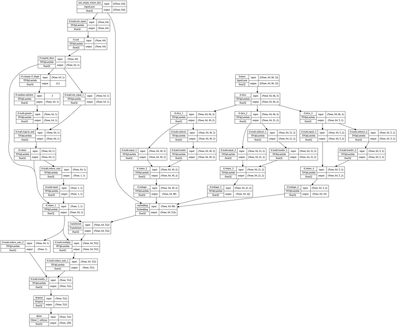
No NaN Predictions
Before training, NaN (Not a Number) values are checked in the predictions made by the model.
if not cfg.PREPROCESS_DATA and cfg.TRAIN_MODEL:
    y_pred = model.predict_on_batch(X_batch).flatten()
    print(f'# NaN Values In Prediction: {np.isnan(y_pred).sum()}')


'''
# NaN Values In Prediction: 0
'''
Weight Initialization
We will be plotting a histogram of the output probabilities of a softmax-initialized model, along with some additional information such as the mean and standard deviation of the probabilities and a red vertical line indicating the baseline probability of random guessing.
if not cfg.PREPROCESS_DATA and cfg.TRAIN_MODEL:
    plt.figure(figsize=(12,5))
    plt.title(f'Softmax Output Initialized Model | µ={y_pred.mean():.3f}, σ={y_pred.std():.3f}', pad=25)
    pd.Series(y_pred).plot(kind='hist', bins=128, label='Class Probability')
    plt.xlim(0, max(y_pred) * 1.1)
    plt.vlines([1 / cfg.NUM_CLASSES], 0, plt.ylim()[1], color='red', label=f'Random Guessing Baseline 1/NUM_CLASSES={1 / cfg.NUM_CLASSES:.3f}')
    plt.grid()
    plt.legend()
    plt.show()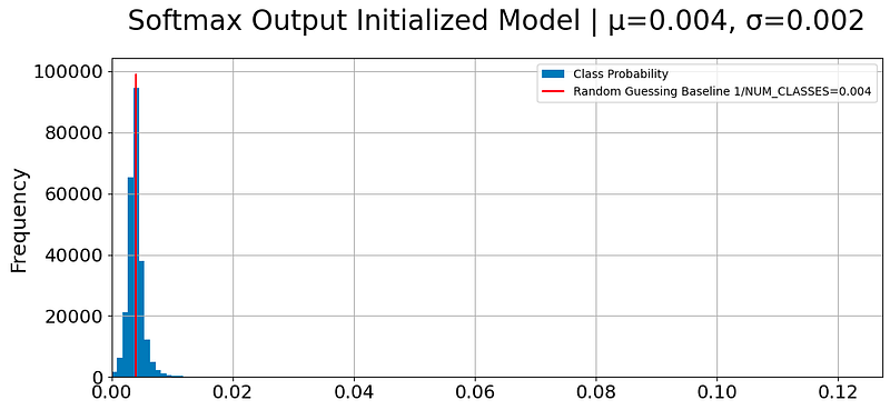
Learning Rate Scheduler
lrfn takes several arguments: “current_step” is the current step number during training, “num_warmup_steps” is the number of steps used for warmup (gradually increasing the learning rate), “lr_max” is the maximum learning rate, “num_cycles” is the number of cycles in the cosine annealing learning rate schedule (default is 0.50), and “num_training_steps” is the total number of training steps.
def lrfn(current_step, num_warmup_steps, lr_max, num_cycles=0.50, num_training_steps=cfg.N_EPOCHS):

    if current_step < num_warmup_steps:
        if cfg.WARMUP_METHOD == 'log':
            return lr_max * 0.10 ** (num_warmup_steps - current_step)
        else:
            return lr_max * 2 ** -(num_warmup_steps - current_step)
    else:
        progress = float(current_step - num_warmup_steps) / float(max(1, num_training_steps - num_warmup_steps))

        return max(0.0, 0.5 * (1.0 + math.cos(math.pi * float(num_cycles) * 2.0 * progress))) * lr_max
The plot_lr_schedule function takes in a learning rate schedule and the total number of epochs and plots the learning rate for each epoch.
def plot_lr_schedule(lr_schedule, epochs):
    fig = plt.figure(figsize=(20, 10))
    plt.plot([None] + lr_schedule + [None])
    # X Labels
    x = np.arange(1, epochs + 1)
    x_axis_labels = [i if epochs <= 40 or i % 5 == 0 or i == 1 else None for i in range(1, epochs + 1)]
    plt.xlim([1, epochs])
    plt.xticks(x, x_axis_labels) # set tick step to 1 and let x axis start at 1

    # Increase y-limit for better readability
    plt.ylim([0, max(lr_schedule) * 1.1])

    # Title
    schedule_info = f'start: {lr_schedule[0]:.1E}, max: {max(lr_schedule):.1E}, final: {lr_schedule[-1]:.1E}'
    plt.title(f'Step Learning Rate Schedule, {schedule_info}', size=18, pad=12)

    # Plot Learning Rates
    for x, val in enumerate(lr_schedule):
        if epochs <= 40 or x % 5 == 0 or x is epochs - 1:
            if x < len(lr_schedule) - 1:
                if lr_schedule[x - 1] < val:
                    ha = 'right'
                else:
                    ha = 'left'
            elif x == 0:
                ha = 'right'
            else:
                ha = 'left'
            plt.plot(x + 1, val, 'o', color='black');
            offset_y = (max(lr_schedule) - min(lr_schedule)) * 0.02
            plt.annotate(f'{val:.1E}', xy=(x + 1, val + offset_y), size=12, ha=ha)

    plt.xlabel('Epoch', size=16, labelpad=5)
    plt.ylabel('Learning Rate', size=16, labelpad=5)
    plt.grid()
    plt.show()

# Learning rate for encoder
LR_SCHEDULE = [lrfn(step, num_warmup_steps=cfg.N_WARMUP_EPOCHS, lr_max=cfg.LR_MAX, num_cycles=0.50) for step in range(cfg.N_EPOCHS)]
# Plot Learning Rate Schedule
plot_lr_schedule(LR_SCHEDULE, epochs=cfg.N_EPOCHS)
# Learning Rate Callback
lr_callback = tf.keras.callbacks.LearningRateScheduler(lambda step: LR_SCHEDULE[step], verbose=1)
Weight Decay Callback
WeightDecayCallback is a custom callback class in TensorFlow Keras that updates the weight decay of the optimizer based on the learning rate. on_epoch_begin method is called at the beginning of each epoch and sets the weight decay of the optimizer to the product of the learning rate and the weight decay ratio. It also prints the learning rate and weight decay for monitoring.
# Custom callback to update weight decay with learning rate
class WeightDecayCallback(tf.keras.callbacks.Callback):
    def __init__(self, wd_ratio=cfg.WD_RATIO):
        self.step_counter = 0
        self.wd_ratio = wd_ratio

    def on_epoch_begin(self, epoch, logs=None):
        model.optimizer.weight_decay = model.optimizer.learning_rate * self.wd_ratio
        print(f'learning rate: {model.optimizer.learning_rate.numpy():.2e}, weight decay: {model.optimizer.weight_decay.numpy():.2e}')
Performance Benchmark
Your model must also perform inference with less than 100 milliseconds of latency per video on average and use less than 40 MB of storage space. Expect to see approximately 40,000 videos in the test set. We allow an additional 10-minute buffer for loading the data and miscellaneous overhead.
%%timeit -n 100
if cfg.TRAIN_MODEL:
    # Verify model prediction is <<<100ms
    model.predict_on_batch({ 'frames': X_train[:1], 'non_empty_frame_idxs': NON_EMPTY_FRAME_IDXS_TRAIN[:1] })
    pass

'''
16.8 ms ± 5.61 ms per loop (mean ± std. dev. of 7 runs, 100 loops each)
'''
Evaluate Initialized Model
We need to verify if the validation dataset covers all signs in the case of USE_VAL mode. The resulting DataFrame from pd.Series.value_counts().to_frame(‘Count’) has rows representing the counts of each unique value in the y_val array. The .iloc function is then used to select specific rows based on their position.
if cfg.USE_VAL:
    # Verify Validation Dataset Covers All Signs
    print(f'# Unique Signs in Validation Set: {pd.Series(y_val).nunique()}')
    # Value Counts
    display(pd.Series(y_val).value_counts().to_frame('Count').iloc[[1,2,3,-3,-2,-1]])
The model.evaluate() function returns the loss value and any specified metrics of the model. *validation_data passes a tuple containing the inputs and outputs of the validation dataset. * is used to unpack the elements of a tuple. The verbose parameter is set to 2, which means no progress updates will be printed during the evaluation.
# Sanity Check
if cfg.TRAIN_MODEL and cfg.USE_VAL:
    _ = model.evaluate(*validation_data, verbose=2)
Train
It creates a fresh model using get_model(), prints a summary of the model’s architecture, and trains the model using model.fit(), which takes various arguments and Keras callbacks for training. The training history is stored in history.
if cfg.TRAIN_MODEL:
    # Clear all models in GPU
    tf.keras.backend.clear_session()


    # Get new fresh model
    model = get_model()

    # Sanity Check
    model.summary()

    # Actual Training
    history = model.fit(
            x=get_train_batch_all_signs(X_train, y_train, NON_EMPTY_FRAME_IDXS_TRAIN),
            steps_per_epoch=len(X_train) // (cfg.NUM_CLASSES * cfg.BATCH_ALL_SIGNS_N),
            epochs=cfg.N_EPOCHS,
            # Only used for validation data since training data is a generator
            batch_size=cfg.BATCH_SIZE,
            validation_data=validation_data,
            callbacks=[
                lr_callback,
                WeightDecayCallback(),
                wandb.keras.WandbCallback()
            ],
            verbose = cfg.VERBOSE,
        )
# Save Model Weights
model.save_weights('model.h5')Validation predictions are performed in the case of USE_VAL mode.
if cfg.USE_VAL:
    # Validation Predictions
    y_val_pred = model.predict({ 'frames': X_val, 'non_empty_frame_idxs': NON_EMPTY_FRAME_IDXS_VAL }, verbose=2).argmax(axis=1)
    # Label
    labels = [ORD2SIGN.get(i).replace(' ', '_') for i in range(cfg.NUM_CLASSES)]
Landmark Attention Weights
We need to retrieve the landmark_weights from the weights of the embedding layer of the model so that we can use the softmax function from the scipy.special module to normalize them. The weights of each of the landmarks (lips, left hand, and pose) indicate how much contribute to the overall recognition model’s decision-making process.
# Landmark Weights
for w in model.get_layer('embedding').weights:
    if 'landmark_weights' in w.name:
        weights = scipy.special.softmax(w)

landmarks = ['lips_embedding', 'left_hand_embedding', 'pose_embedding']

for w, lm in zip(weights, landmarks):
    print(f'{lm} weight: {(w*100):.1f}%')


'''
lips_embedding weight: 28.5%
left_hand_embedding weight: 46.8%
pose_embedding weight: 24.7%
'''
Classification Report
The classification report uses sklearn.metrics.classification_report function, which takes in the true labels y_val, predicted labels y_val_pred, target names (labels) of the classes, and an argument output_dict=True to return the report as a dictionary.
def print_classification_report():
    # Classification report for all signs
    classification_report = sklearn.metrics.classification_report(
            y_val,
            y_val_pred,
            target_names=labels,
            output_dict=True,
        )
    # Round Data for better readability
    classification_report = pd.DataFrame(classification_report).T
    classification_report = classification_report.round(2)
    classification_report = classification_report.astype({
            'support': np.uint16,
        })
    # Add signs
    classification_report['sign'] = [e if e in SIGN2ORD else -1 for e in classification_report.index]
    classification_report['sign_ord'] = classification_report['sign'].apply(SIGN2ORD.get).fillna(-1).astype(np.int16)
    # Sort on F1-score
    classification_report = pd.concat((
        classification_report.head(cfg.NUM_CLASSES).sort_values('f1-score', ascending=False),
        classification_report.tail(3),
    ))

    pd.options.display.max_rows = 999
    display(classification_report)

if cfg.USE_VAL:
    print_classification_report()
This code resulted in a score of 0.72 on the leaderboard.
I hope this article is helpful for you. Thank you for reading :D